
Excel for iPad recently added the ability to create pivot tables, allowing users to easily analyze and summarize their data. The official one was updated today Microsoft Excel blog. The blog says that the iPad version of Excel now supports pivot tables.

The company announced the following in a blog:
"My happy to inform about support creation and editing summary tables on the iPad. Raised tables allow calculate, summarize and analyze data. My adapted this a powerful tool for the iPad's smaller screen and touch interface. Now you can easily move between desktop computer, Internet and iPad, keeping with unchanged quality of work. Open the whole the potential of pivot tables, making every calculation and analysis simple and comfortable under way"
Excel for iPad users can create a new PivotTable by opening the Insert tab and selecting the PivotTable option. Users can then select an insertion source and location to insert their pivot table onto the iPad touchscreen. Users can also change the data source in the PivotTable report by clicking the Change Data Source option. This will bring up a sidebar where changes can be made, and users can also click on the “Settings” sidebar to fine-tune the pivot table information. Pivot tables are powerful data calculation, summarization, and analysis tools that help you see comparisons, patterns, and trends in your data. We may use pivot tables to calculate data based on certain criteria. For example, sales per store, sales per year, average discounts in the region, etc.
How to create a pivot table
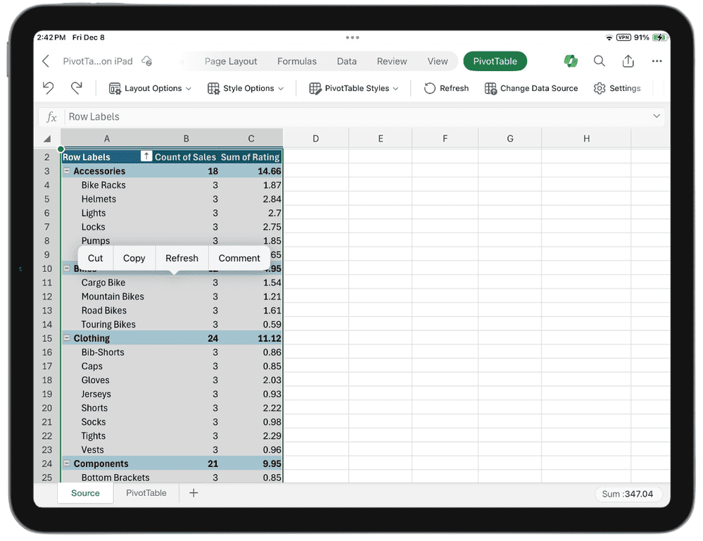
Here's a step-by-step guide from Microsoft on how to create a pivot table on the iPad
1. Creating a summary table
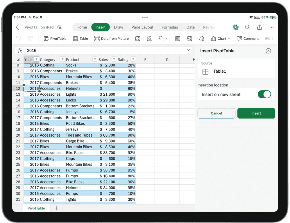
To create a pivot table, go to the Insert tab at the top of the screen and click Pivot Table. then select “Source” and “Insert Location” and insert the pivot table with one click.
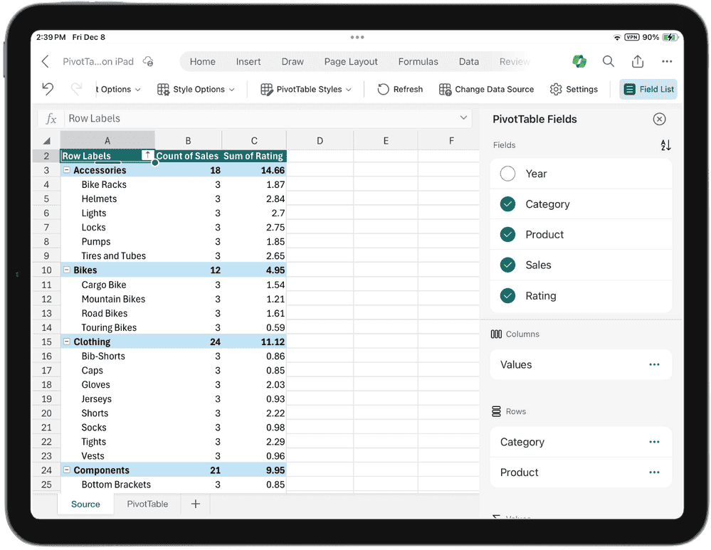
2. Using the list of fields
With the field list, you can easily customize the pivot table the way you need it. The lower Areas section allows you to easily rearrange fields by dragging them between different sections to get an intelligent view of the data.
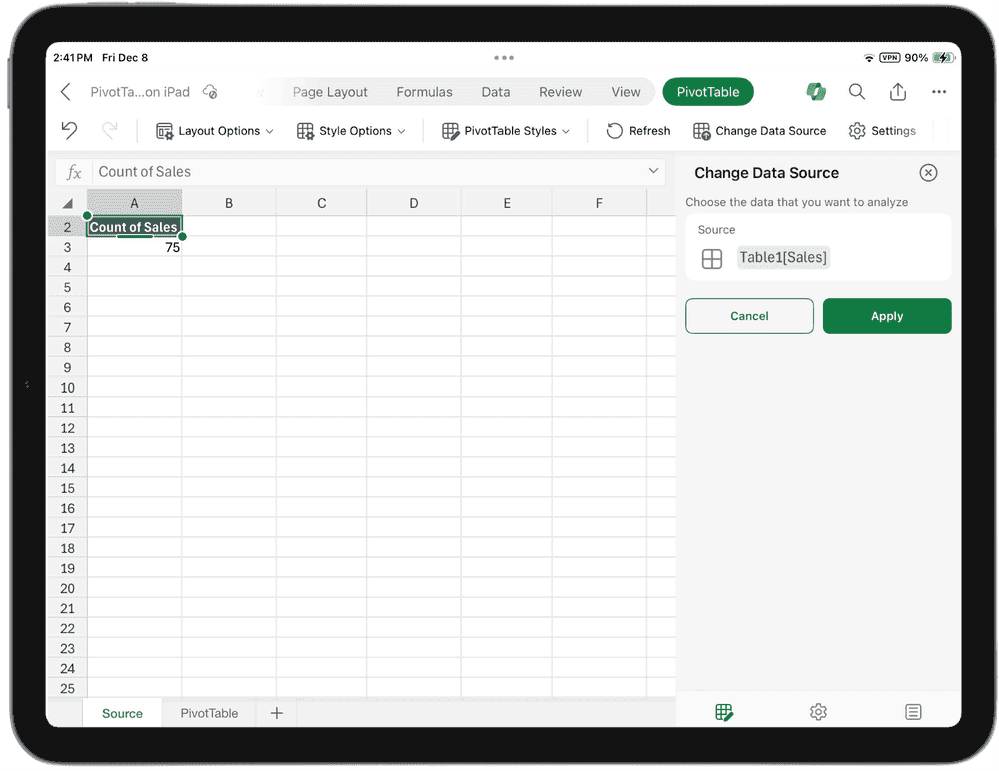
3. Change the output data
Go to the PivotTable tab and select the Change Data Source sidebar to make changes to the PivotTable output data. It's a simple process that ensures your analysis is dynamic and relevant.
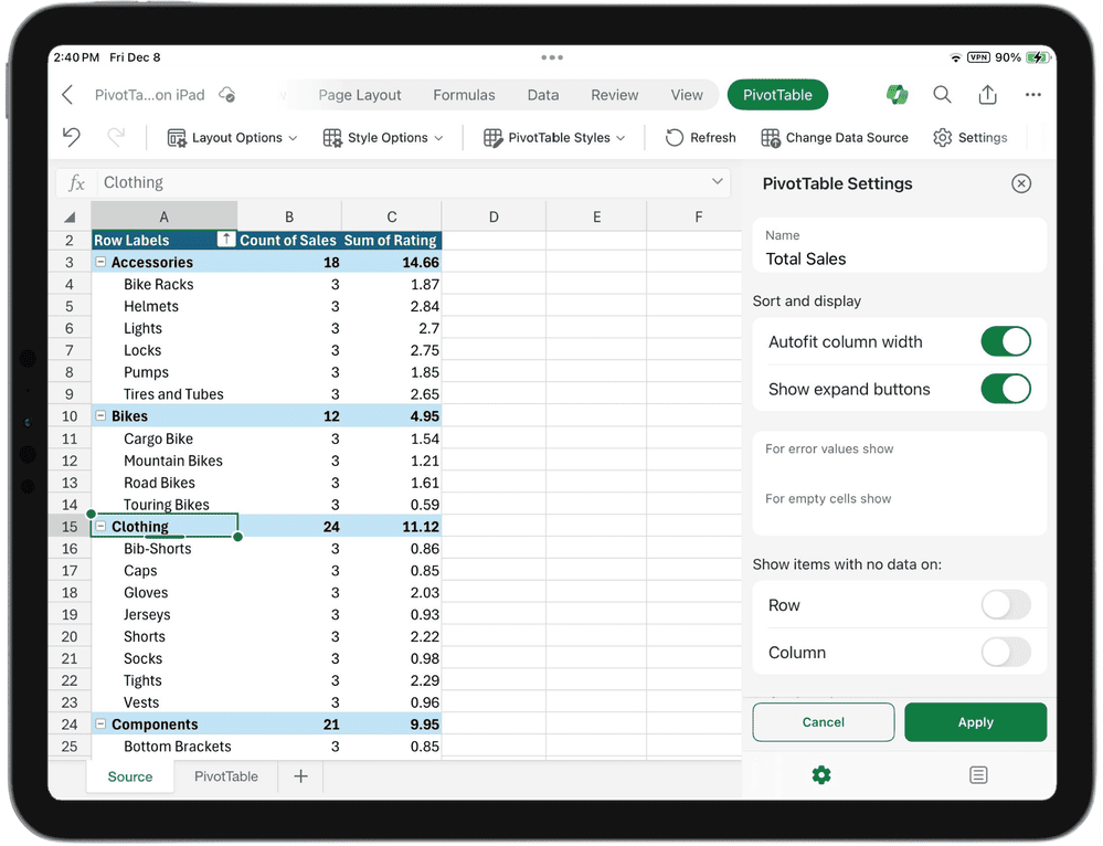
4. Change settings
Go to the “Settings” sidebar to easily customize your pivot table. Make the necessary changes and save them with one tap to make sure your pivot table works exactly the way you want it to.
5. Moving the summary table
Cut and paste from the context menu to move the pivot table within a sheet or between sheets.
Other ways to use a pivot table on iPad
Prior to the official introduction of PivotTables for iPad, Excel for iPad did not support creating new PivotTables directly in the app. Instead, users had to either create a pivot table in Office on the web or use an alternative workaround. One such way is to remove Excel from the iPad and log in to Office.com through a web browser. If you don't have an update that allows you to create pivot tables on iPad, you can still try the old solution below
Creating pivot tables in Excel for iPad
As we said earlier, you cannot create a new pivot table, but you can work with existing pivot tables in the file. To create a pivot table in Excel for iPad, you'll need Office on the Web. It can be accessed through a web browser by signing in with a Microsoft account. Once signed in, select Excel and follow the steps below
Summary tables with subheadings
Although Excel for iPad does not yet support creating pivot tables with subheadings, Office on the web allows you to create and modify pivot tables with subheadings. To create a pivot table with subheadings in Excel for iPad, follow these steps:
- Sign in to Office.com through a web browser on iPad.
- Select Excel and create a new worksheet or open an existing one.
- Go to the “Insert” tab and select “Pivot Table”
A new update for Excel on iPad now supports this feature. For this reason, users do not need to use a log workaround to use this feature. Users expressed their desire for this feature and Microsoft listened to them and now it is available.
Visnovok
Microsoft has just announced that Excel on iPad now supports pivot tables. This is a feature that many people, especially scientists, have longed for. It is not always convenient to switch to a laptop when you need to work with a summary table. Users can now create and modify pivot tables on their iPads with just a few clicks. Those who have not yet upgraded can create and modify pivot tables with subheadings using Office on the Web. They can also import this table to the iPad and modify it.